World Models & Vision-Language-Action Models: An Advanced Field Guide
A technical survey of how machines learn to simulate and act in the physical world from Sutton's Dyna to pi-0 and Dreamer 4 covering architectures, math, and open problems.
A structured tour through the papers, systems, and ideas that define how machines learn to understand and act in the physical world: from foundational theory to the frontier.
Contents#
Part I. Foundations: The Intellectual Roots (1990–2022)
- I1. Learning a model, then planning inside it
- I2. The world model renaissance
- I3. Yann LeCun's manifesto and the JEPA vision
Part II. World Models: Learning to Simulate Reality (2018–Now)
- Part II1. Latent imagination: the Dreamer line
- Part II2. Planning with learned dynamics: MuZero and TD-MPC
- Part II3. Joint Embedding Predictive Architectures (JEPA)
- Part II4. Video generation as world simulation
- Part II5. Evaluating world models
- Part II6. Pause. Where are the surveys?
Part III. Vision-Language-Action Models: From Understanding to Doing (2022–Now)
- Part III0. What even is a VLA?
- Part III1. The RT series and the birth of the paradigm
- Part III2. Open-source VLAs that changed the game
- Part III3. Industry VLAs pushing the frontier
- Part III4. Architectures and action decoders: a design space
Part IV. Core Methodologies: The Building Blocks
- Part IV1. Imitation learning's watershed moment
- Part IV2. Action tokenization and representation
- Part IV3. Chain-of-thought reasoning for robots
- Part IV4. 3D and spatial representations
Part VI. Open Challenges and What Comes Next
Awesome Lists & Living Resources
Part I. Foundations: The Intellectual Roots (1990–2022)#
I1. Learning a model, then planning inside it#
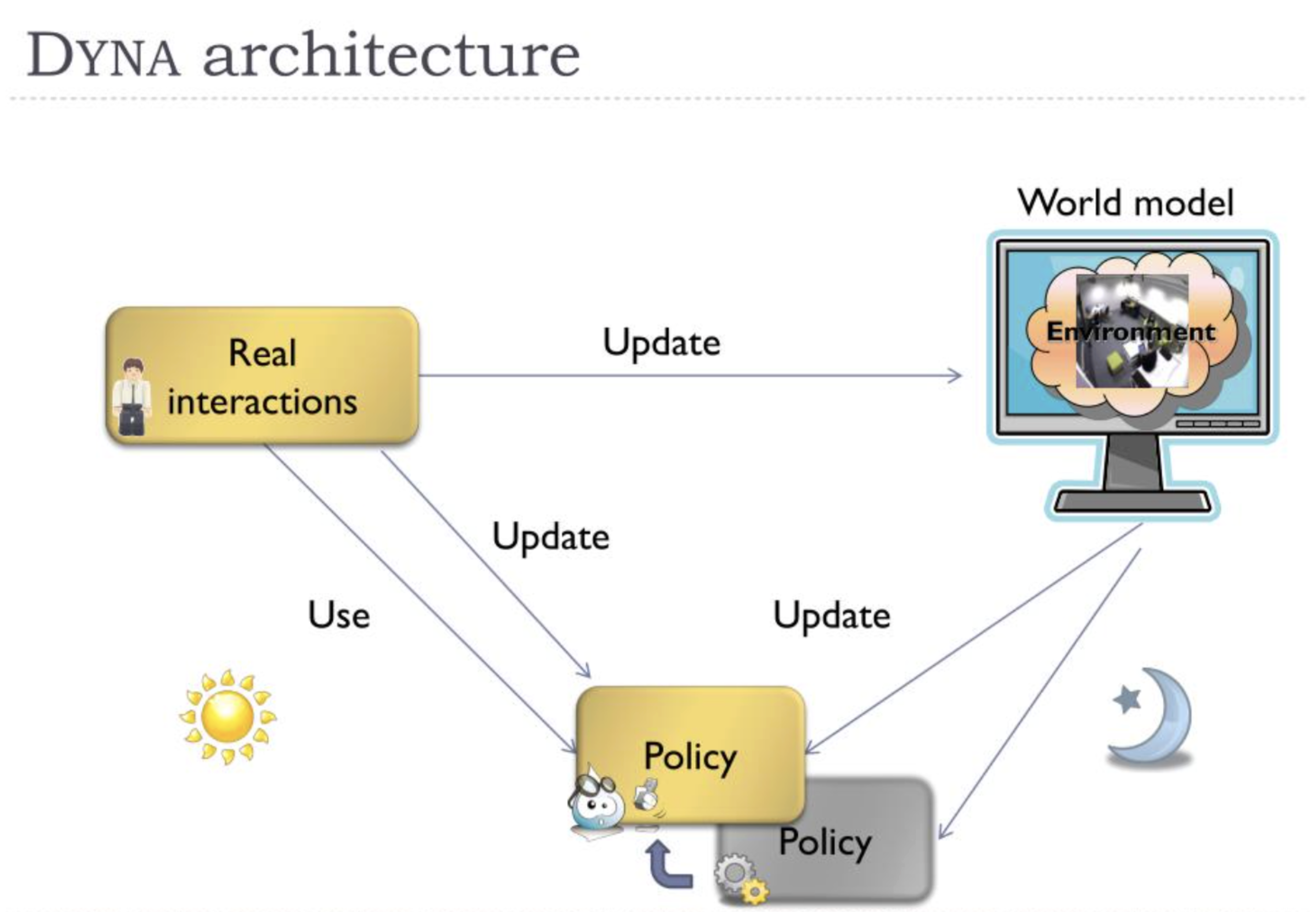
The idea of a world model is older than deep learning. In 1990, Richard Sutton introduced the Dyna architecture [1], which proposed a strikingly clean separation: an agent learns a model of its environment from real experience, then uses that model to generate imagined experience for planning.
Architecturally, Dyna is simple. The agent maintains three components: a policy (mapping states to actions), a value function (estimating future reward), and a model (predicting the next state and reward given a state-action pair). On every real time step, the agent (1) takes an action in the environment and observes the result, (2) updates the model with this new tuple, and (3) performs additional "planning steps" by sampling previous states, querying the model for predicted transitions, and using those imaginary transitions to update the policy and value function via standard temporal-difference learning. The ratio of planning steps to real steps is the knob that controls how much you learn from imagination vs. reality.
┌──────────────────────────────────────────────────────┐
│                   DYNA ARCHITECTURE                  │
│                                                      │
│   Real Environment                                   │
│        │                                             │
│        ▼                                             │
│   ┌─────────┐   (s, a, s', r)   ┌────────────────┐   │
│   │  Agent  │──────────────────►│ Learned Model  │   │
│   │ (Policy │                   │  M(s,a)→(r,s') │   │
│   │  + Q)   │◄──────────────────│                │   │
│   └─────────┘   k planning      └────────────────┘   │
│        │         steps using                         │
│        │         simulated                           │
│        ▼         experience                          │
│   Take action                                        │
│   in real env                                        │
└──────────────────────────────────────────────────────┘
The core update rule is the same for both real and simulated transitions. Given any transition , whether from the real environment or the learned model , the Q-learning update is:
Reading this equation: The agent updates its estimate of how good it is to take action in state . The term in brackets is the temporal difference (TD) error: it compares the observed reward plus the discounted best future value against the current estimate . The learning rate controls how fast estimates update; the discount controls how much the agent cares about the future. The key insight is that this identical update works whether came from the real world or was hallucinated by the model.
The formal equivalence is that both the "direct RL" path (real experience) and the "planning" path (model-generated experience) minimize the same Bellman error , just with different data sources. In the model-free limit (), Dyna reduces to standard Q-learning. As , it approaches full value iteration using the learned model.
Prioritized Sweeping (Moore & Atkeson, 1993) improved upon Dyna's random sampling of planning steps by maintaining a priority queue ordered by TD error magnitude. When a transition produces large , the algorithm propagates backward: for all predecessor pairs predicted to lead to , it computes the expected TD error and inserts them into the queue if . This backward-chaining ensures value changes propagate efficiently, often requiring orders of magnitude fewer updates than uniform sampling.
This exact structure: real data collection, model update, imagined rollouts for policy improvement, recurs in DreamerV3, TD-MPC, and virtually every model-based RL system since. The formal relationship: model-free learning applies the Bellman optimality operator using samples from the true MDP transition kernel , while model-based planning applies using samples from the approximate model . If you read one paper from before 2010, make it this one.
I2. The world model renaissance#
The modern revival came in 2018 when Ha and Schmidhuber published "World Models" [2]. Their architecture is a three-stage pipeline, and understanding it precisely clarifies a lot of what came later:
┌─────────────────────────────────────────────────────────────┐
│              HA & SCHMIDHUBER WORLD MODELS                  │
│                                                             │
│  Pixels ──► [V: VAE] ──► z_t ──► [M: MDN-RNN] ──► z_t+1.    │
│              64x64        32d       LSTM+MDN     predicted  │
│                            │                                │
│                            ▼                                │
│                    [C: Linear Controller]                   │
│                      z_t + h_t ──► a_t                       │
│                      (867 parameters)                         │
│                                                             │
│  Training:  V trained on pixels (VAE loss)                  │
│             M trained on latent sequences (NLL)             │
│             C trained entirely in M's dream (CMA-ES)        │
└─────────────────────────────────────────────────────────────┘
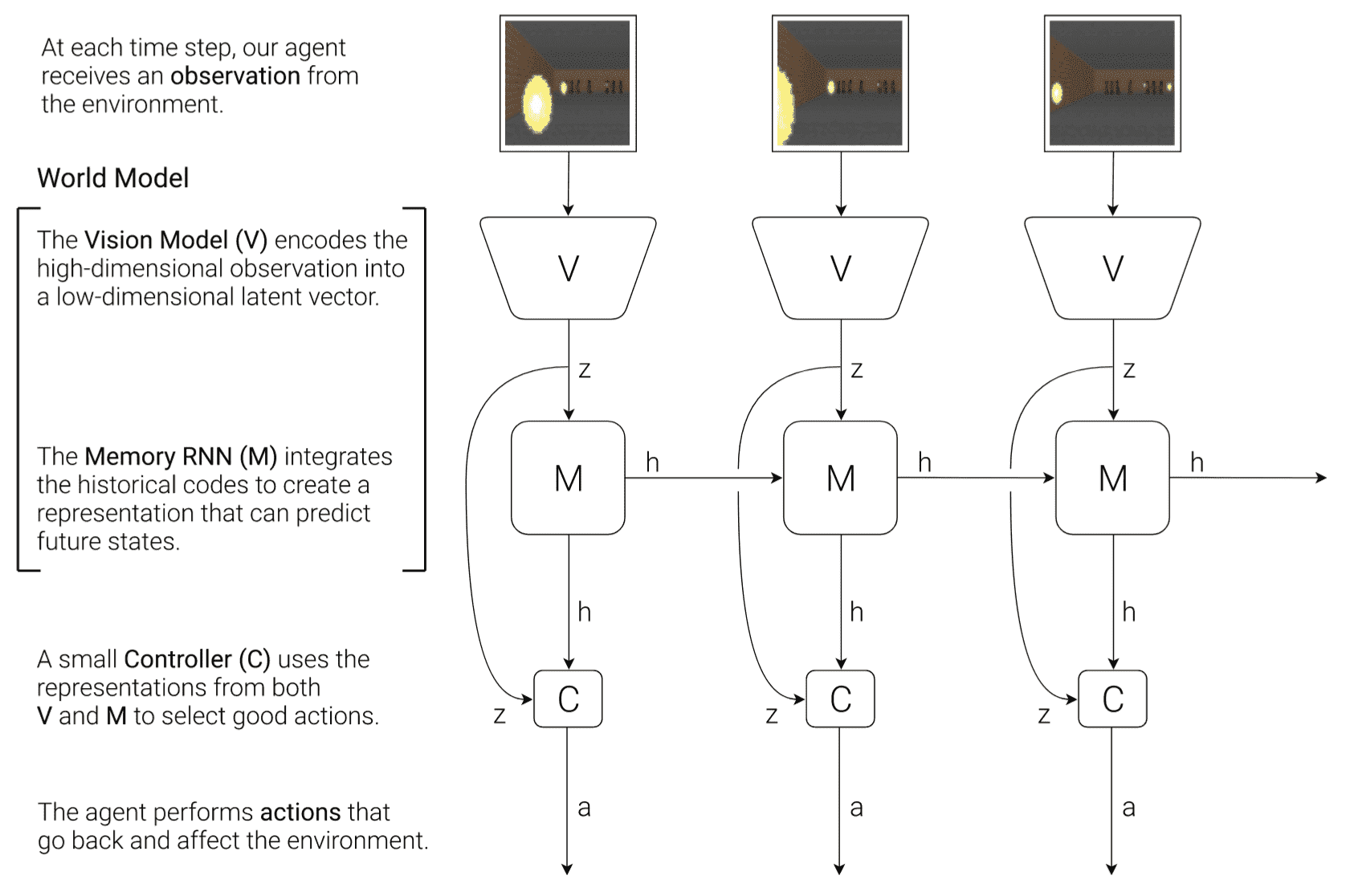
- Vision model (V): A Variational Autoencoder (VAE) compresses each RGB observation frame into a small latent vector . The encoder maps pixels to latent, and the decoder maps latent to pixels. The VAE is trained by maximizing the Evidence Lower Bound (ELBO):
Reading this equation: The VAE loss has two competing terms. The first term is the reconstruction quality: how well can the decoder reproduce the original image from the latent code ? The second term is the regularization penalty: it forces the encoder's output distribution to stay close to a simple standard Gaussian . This tension produces a smooth, structured latent space where nearby points decode to similar images.
The encoder is , the decoder is , and the prior is . The KL term has a closed-form solution for two Gaussians:
Reading this equation: For each of the latent dimensions, the KL divergence measures how far the encoder's mean and variance are from the standard normal (mean 0, variance 1). If and , this term is zero: the encoder already matches the prior.
- Memory model (M): A Mixture Density Network layered on top of an LSTM (MDN-RNN) takes the current latent and action and predicts a probability distribution over the next latent . For each latent dimension , the output is a Gaussian mixture with components:
Reading this equation: Rather than predicting a single next state, the model predicts a mixture of possibilities. Each component has a weight (how likely this mode is), a mean (the predicted value), and a variance (how uncertain it is). For example, if a ball could bounce left or right, one component captures "bounce left" and another "bounce right," each with its own probability. The components give the model enough flexibility to represent stochastic, multi-modal transitions.
The network outputs parameters per dimension: mixing coefficients (through softmax so ), means , and log-standard-deviations . The total loss is the negative log-likelihood:
Reading this equation: The model is trained to maximize the likelihood of the actually observed next latent under the predicted mixture distribution. Negative log-likelihood turns this into a minimization problem. Summing over time and dimensions means the model is trained across the full sequence and all latent dimensions jointly.
A temperature parameter scales the mixture standard deviations at sampling time (), controlling the stochasticity of dreamed rollouts. This is the world model proper: given where you are and what you do, it predicts what will happen next.
- Controller (C): A simple linear controller maps the concatenation of and the hidden state of the RNN to an action:
Reading this equation: This is just a linear transformation: concatenate the 32-dim latent code with the 256-dim RNN hidden state , multiply by a weight matrix , and add a bias . With and , this yields only parameters (e.g., 867 for a 3-dimensional action space). The controller is deliberately tiny: the entire intelligence lives in the world model, and the controller just exploits it.
It is optimized with Covariance Matrix Adaptation Evolution Strategy (CMA-ES), which maintains a multivariate Gaussian search distribution over the parameter vector. At each generation , it samples candidates, evaluates their fitness (cumulative reward), selects the top performers, and updates the mean and covariance:
Reading this equation: CMA-ES evolves a population of candidate controllers. The new mean is a weighted average of the best-performing solutions (ranked by fitness). The covariance adapts the search shape: the first term carries forward the old covariance, the second term uses the evolution path (a momentum-like cumulated step direction) to stretch the search along successful directions, and the third term updates using the spread of top solutions. This is gradient-free optimization: no backpropagation needed, which avoids differentiating through the stochastic MDN-RNN rollouts.
The provocative result: by training the controller entirely inside the M model's dream (rolling out the MDN-RNN without any real environment interaction), the agent learned to play VizDoom and car racing tasks. The agent was literally trained in its own hallucination. This paper established two principles that persist: (a) compress observations into a learned latent space, and (b) learn dynamics in that latent space, not in pixel space.
I3. Yann LeCun's manifesto and the JEPA vision#
In 2022, Yann LeCun published "A Path Towards Autonomous Machine Intelligence" [3], which reframed the entire conversation. His argument targets a specific architectural choice: generative models that predict pixels (or any high-dimensional output) are wasteful because they must model every irrelevant detail: the exact texture of a leaf, the precise pattern of shadows. Instead, he proposed Joint Embedding Predictive Architectures (JEPA), which work in representation space.
┌────────────────────────────────────────────────────────────┐
│                JEPA vs. GENERATIVE MODEL                   │
│                                                            │
│  Generative (pixel prediction):                            │
│    Image ──► Encoder ──► z ──► Decoder ──► Predicted Image │
│    Loss = ||pixels - predicted_pixels||                    │
│    Must reconstruct every detail (noise, texture, etc.)    │
│                                                            │
│  JEPA (representation prediction):                         │
│    Context ──► Context Encoder ──► s_x                     │
│                                     │                      │
│                               ┌─────▼──────┐               │
│    Target ──► Target Encoder  │  Predictor │               │
│               (EMA copy) ──►  │  g(s_x, z) │               │
│               s_y             └─────┬──────┘               │
│                                     │                      │
│    Loss = ||s_y - predicted_s_y||                          │
│    Free to ignore irrelevant details                       │
└────────────────────────────────────────────────────────────┘
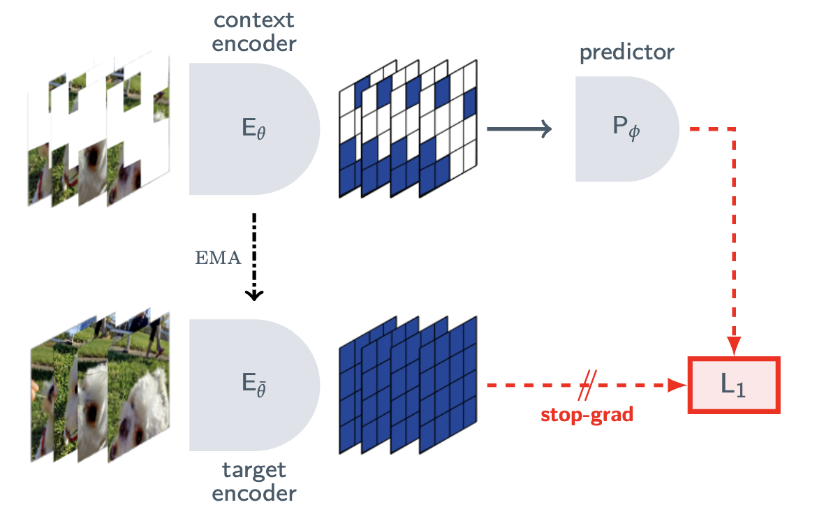
The JEPA architecture has two branches. A context encoder processes the observed portion of the input (e.g., visible patches of an image) and produces a representation . A predictor takes this representation plus a specification of what to predict (e.g., the location of masked patches) and outputs a predicted representation , where is a latent variable. A target encoder (often an exponential moving average of the context encoder, a la BYOL/DINO) processes the actual target portion and produces the ground-truth representation . The training objective minimizes the distance between the predicted and target representations in embedding space: never in pixel space.
The critical challenge is representational collapse: the system can trivially minimize prediction error by mapping all inputs to a constant. JEPA-family methods prevent this through non-contrastive mechanisms. The VICReg objective (Bardes et al., 2022) provides one such mechanism, combining three terms:
Reading this equation: VICReg prevents collapse with three forces. Invariance : pulls representations of matched pairs together (minimize distance). Variance : pushes each embedding dimension to maintain a minimum spread across the batch (prevents collapsing to a single point). Covariance : decorrelates dimensions (prevents collapsing to a low-dimensional subspace). The hyperparameters balance these competing objectives, with typical values (variance prevention is weighted heavily).
The three terms in detail:
- Invariance:
- Variance: with threshold
- Covariance: where
The EMA target encoder provides an alternative collapse-prevention mechanism. The target encoder is not trained by gradient descent but tracks the online encoder via:
Reading this equation: After each training step, the target encoder's weights are updated as a weighted average: fraction of its old weights plus fraction of the online encoder's current weights . With (very close to 1), the target encoder changes extremely slowly, creating a stable prediction target. This asymmetry: the online network chases a slowly-moving target, prevents both networks from collapsing to trivial solutions together.
The loss is where denotes stop-gradient. Analysis by Tian et al. (2021) shows the online predictor breaks symmetry: without it, even EMA targets collapse.
The crucial consequence: the model is free to discard information that is not predictable or not useful. Pixel-level generative models must reconstruct noise, texture, and irrelevant detail. JEPA models can learn to focus only on the structure and semantics that matter for downstream tasks. This distinction: predict pixels vs. predict representations, became the defining tension of the field. Meta's entire V-JEPA line follows directly from this manifesto, while OpenAI (Sora) and DeepMind (Genie) bet on the generative approach.
Separately, Taniguchi et al. [4] bridged neuroscience and AI by surveying predictive coding, the free-energy principle, and active inference in the context of cognitive and developmental robotics. Friston's Free Energy Principle provides the formal framework: any self-organizing system at equilibrium with its environment must minimize variational free energy , an upper bound on surprisal:
Reading this equation: Free energy is an upper bound on surprisal (how unexpected observations are). The energy term measures how well the agent's internal model explains observations: if internal beliefs about hidden causes poorly predict what was observed, this term is large. The complexity term penalizes beliefs that deviate too far from prior expectations : Occam's razor built into the math. Minimizing with respect to beliefs = perception (updating your model of the world). Minimizing with respect to actions = active inference (acting to make the world match your predictions). This unifies perception and action under a single variational objective.
In hierarchical predictive coding networks, prediction errors at each cortical level are weighted by precision , and the total free energy sums precision-weighted squared errors across all levels. The connection to Dyna is direct: Sutton's agent learns a model and plans inside it; the brain (per this theory) does the same thing, but the planning and perception are unified under a single variational objective.
Part II. World Models: Learning to Simulate Reality (2018–Now)#
Part II1. Latent imagination: the Dreamer line#
The Dreamer series from Danijar Hafner and collaborators represents the most sustained and successful effort to build general-purpose latent world models. Each iteration made a specific architectural bet that paid off.
DreamerV1 (2020) [5] introduced the Recurrent State-Space Model (RSSM), which remains the core engine of the entire line. The RSSM maintains two types of state: a deterministic recurrent state (the hidden state of a GRU, capturing long-term memory) and a stochastic state (sampled from a learned prior, capturing uncertainty). The combined model state at time is the pair .
┌───────────────────────────────────────────────────────────┐
│                    RSSM ARCHITECTURE                      │
│                                                           │
│                    ┌───────────┐                          │
│    a_{t-1} ───────►│           │                          │
│    z_{t-1} ───────►│  GRU Cell │───────► h_t              │
│    h_{t-1} ───────►│           │          │               │
│                    └───────────┘          │               │
│                                           │               │
│                    ┌─────────────────────┐│               │
│   Prior:           │  p(z_t | h_t)       ││  (imagination)│
│   (no observation) └─────────────────────┘│               │
│                                           │               │
│                    ┌─────────────────────┐│               │
│   Posterior:       │ q(z_t | h_t, o_t)   ││  (training)   │
│   (with obs o_t)   └─────────────────────┘│               │
│                                           │               │
│                           h_t + z_t ──────┤               │
│                               │           │               │
│                     ┌─────────▼──┐  ┌─────▼─────┐         │
│                     │  Decoder   │  │  Reward   │         │
│                     │  ô_t       │  │  r̂_t      │         │
│                     └────────────┘  └───────────┘         │
└───────────────────────────────────────────────────────────┘
The RSSM is defined by four components:
Deterministic state update (recurrence):
Reading this equation: The GRU cell takes the previous deterministic state , previous stochastic state , and the action taken , and produces the new deterministic state . This is the "memory backbone" that carries persistent information forward in time.
Stochastic prior (transition predictor):
Reading this equation: The prior predicts what might happen next using only the deterministic memory , without looking at the current observation. This is what the model uses during imagination (dreaming), when no real observations are available.
Stochastic posterior (representation model):
Reading this equation: The posterior incorporates the actual observation (encoded via a CNN ) to produce a more informed estimate. During training with real data, the posterior provides better state estimates. The gap between prior and posterior (measured by KL divergence) is what drives the prior to improve.
Observation decoder and reward predictor:
Reading this equation: From the combined state , the model reconstructs observations and predicts rewards . These reconstruction signals provide the training gradients that force the latent states to encode meaningful information about the world.
The full model is trained by maximizing the ELBO on the observation and reward sequence. For a sequence of length :
Reading this equation: Three terms summed at every timestep. The reconstruction term rewards the model for accurately predicting observations from its latent state. The reward prediction term rewards it for predicting rewards. The KL regularizer penalizes the posterior for diverging from the prior : this trains the prior to match the posterior, which is critical because during imagination (planning), only the prior is available. The weight controls the prior/posterior trade-off.
The key innovation over Ha & Schmidhuber [2] is that the stochastic and deterministic paths are entangled: the GRU carries forward persistent memory while the stochastic state models per-step uncertainty, and the entire thing is trained end-to-end via variational inference.
DreamerV2 (2021) [6] made a seemingly small but consequential change: switching the stochastic state from a Gaussian to a categorical distribution: specifically, 32 categorical variables each with 32 classes:
Reading this equation: Instead of sampling from a continuous Gaussian, each of the 32 stochastic variables is independently drawn from a 32-class categorical distribution (like rolling 32 independent 32-sided dice). This creates a discrete codebook with possible states. Straight-through gradients allow backpropagation. The intuition: categoricals avoid the pathology of Gaussian posteriors collapsing to the prior (posterior collapse), and they naturally encourage distinct, interpretable state codes.
DreamerV2 also introduced KL balancing, which separately weights the KL gradient to the posterior vs. the prior:
Reading this equation: With , 80% of the gradient trains the prior to match the posterior ( = stop-gradient, so the posterior is treated as fixed), and only 20% pushes the posterior toward the prior. This asymmetry prevents the posterior from being overly regularized, which would discard observation information. Without balancing, the KL term can suppress the posterior too aggressively, collapsing it to match a poor prior.
DreamerV2 achieved human-level performance on 55 Atari games from raw pixels.
DreamerV3 (2025, published in Nature) [7] is the reference paper for anyone building systems. Its core contribution is robustness across domains without hyperparameter tuning. The key architectural additions:
(a) Symlog predictions, which apply a symmetric logarithmic transformation to targets:
Reading this equation: Symlog compresses large magnitudes logarithmically while remaining approximately linear near zero ( for ). It preserves sign and is differentiable everywhere. A reward of 10,000 becomes , while a reward of 0.01 stays . This lets a single loss function handle rewards spanning many orders of magnitude without clipping or per-task normalization.
The loss is computed in transformed space: , with inverse . DreamerV3 applies symlog to both the reward model and the critic's value function, predicting a categorical distribution over a symlog-transformed discrete support ("twohot" encoding over 255 bins spanning in symlog space).
(b) Free bits for the KL loss: with nat, preventing posterior collapse by only penalizing KL divergence above a minimum threshold.
(c) A return normalization scheme that adapts to the scale of returns automatically.
The result is a single set of hyperparameters that works across Atari, continuous control (DMC), Minecraft, Crafter, and more.
Dreamer 4 (September 2025) [8] replaced the RSSM's GRU backbone with a transformer architecture, enabling much longer context windows and better scaling. The headline result: solving the Minecraft Diamond Challenge (20,000+ sequential actions from raw pixels) from purely offline data. This required two key innovations. First, shortcut forcing: during training, the model is asked to predict future states at varying temporal strides (1 step, 4 steps, 16 steps ahead), which forces it to learn multi-scale dynamics and prevents the model from only being accurate at single-step predictions. Second, an efficient attention mechanism that allows real-time interactive inference on a single GPU. The offline-only setting is significant: it means the model learns world dynamics entirely from pre-recorded video, never interacting with Minecraft during training.
Part II2. Planning with learned dynamics: MuZero and TD-MPC#
A parallel line of work focuses on using learned models for planning at test time, rather than for imagination-based policy training during learning.
MuZero (2020) [9] from DeepMind takes an elegant stance: it learns a dynamics model, but this model never reconstructs observations. Instead, it operates entirely in an abstract latent space and is trained end-to-end to be useful for planning. The architecture has three components:
┌────────────────────────────────────────────────────┐
│                  MuZero ARCHITECTURE               │
│                                                    │
│  Real obs ──► h_θ (Representation) ──► s^0         │
│                                         │          │
│               ┌─────────────────────────┤          │
│               │                         │          │
│               ▼                         ▼          │
│         f_θ (Predict)           g_θ (Dynamics)     │
│         s^k → (p^k, v^k)       (s^k, a^k) → s^k+1. │
│         policy + value          + reward r^k       │
│                                                    │
│  Key: Hidden states s^k have NO pixel grounding.   │
│  They are trained purely to support planning.      │
└────────────────────────────────────────────────────┘
- Representation function : maps a real observation to an initial hidden state .
- Dynamics function : given a hidden state and an action, predicts the next hidden state and immediate reward: .
- Prediction function : given a hidden state, predicts a policy distribution and value: .
At test time, MuZero runs Monte Carlo Tree Search (MCTS): starting from the current real state, it expands a search tree. Each of simulations (typically –) consists of three phases:
(1) Selection. At each internal node, actions are chosen to maximize the PUCT score:
Reading this equation: PUCT balances exploitation and exploration. The first term is the current estimated value (exploit what you know is good). The second term combines the neural network's prior with an exploration bonus that is large for rarely-visited actions and shrinks as an action is explored more. The coefficient grows slowly with total visits, maintaining exploration even as the tree deepens. Q-values are normalized to using .
(2) Expansion. At a leaf node, the dynamics function produces the new state and reward, and produces the policy prior and value.
(3) Backup. Values are backed up along the path with discounted cumulative rewards:
Reading this equation: The return at depth sums discounted rewards from step down to the leaf at depth , then adds the discounted leaf value as a bootstrap estimate of future returns beyond the search horizon.
Loss Functions. MuZero is trained on trajectories from a replay buffer. For each sampled position , the model unrolls hypothetical steps:
Reading this equation: Three losses are summed at each of imagined steps. The policy loss trains the prediction function to match the MCTS-improved policy (visit count distribution: ). The value loss trains value predictions to match bootstrapped -step returns . The reward loss trains reward predictions to match actual observed rewards . The regularizer prevents overfitting. Gradients are scaled by when passing through the dynamics function to maintain stability across the unrolled steps.
Relationship to AlphaZero. AlphaZero is a special case where the representation function is the identity on the board state, the dynamics function is replaced by the known perfect game simulator, and the reward head is unnecessary. MuZero's contribution is replacing the perfect simulator with a learned model while maintaining MCTS.
The contrast with Dreamer is fundamental. Dreamer learns an explicit latent simulator and trains a policy offline by rolling it out. MuZero learns an implicit latent simulator and uses it online via search. Dreamer is better for continuous control; MuZero is better for discrete, combinatorial domains.
TD-MPC (2022) [10] brought model-based planning to continuous control. It learns a latent dynamics model and uses it with Model Predictive Path Integral (MPPI) planning: a sampling-based method rooted in the path integral formulation of stochastic optimal control.
┌────────────────────────────────────────────────┐
│                MPPI PLANNING                   │
│                                                │
│  Current state z_0                             │
│       │                                        │
│       ├──► Sample N perturbed action sequences │
│       │    a_i^k = π(z_i^k) + ε_i^k            │
│       │                                        │
│       ├──► Roll out each through dynamics model│
│       │    Compute cost S_i for each           │
│       │                                        │
│       ├──► Softmax-weight by -S_i / λ          │
│       │                                        │
│       └──► Update plan: μ^k += Σ w_i ε_i^k     │
│            Execute μ^0                         │
└────────────────────────────────────────────────┘
The MPPI procedure:
- Sample action perturbations: for and .
- Form candidate actions: , biased toward the learned policy prior: .
- Roll out each sequence through the learned dynamics model to compute costs, including a learned terminal value:
Reading this equation: The total cost for trajectory sums discounted negative rewards (negative because MPPI minimizes cost, not maximizes reward) over the planning horizon , then adds the discounted negative Q-value at the terminal state as a bootstrap. This terminal value is the key ingredient allowing short horizons (–) to capture long-term consequences.
- Compute importance weights using the softmax of negative costs:
Reading this equation: Each trajectory gets a weight proportional to . Lower cost = higher weight. The temperature controls sharpness: small concentrates weight on the best trajectories (greedy), large spreads weight more evenly (more exploration).
- Update the mean plan: . Execute .
TD-MPC2 (2024) [11] scaled this to multi-task settings with a single model across 104 continuous control tasks. Key improvements: normalizing the latent state to the unit hypersphere (), using symlog-transformed targets, and a consistency loss:
Reading this equation: The predicted next latent must match the encoded actual next observation (via an EMA target encoder, stop-gradiented). This "consistency" loss grounds the latent dynamics in reality: without it, the latent states could drift to represent something useful for value prediction but disconnected from actual observations.
Part II3. Joint Embedding Predictive Architectures (JEPA)#
Following LeCun's manifesto [3], Meta's research line developed the JEPA framework into concrete systems, progressively scaling from images to video to action.
I-JEPA (ICCV 2023) [12] operates on images. The architecture masks a large portion of an image (typically 75-90%) and predicts the representations of the masked patches from visible context. The context encoder is a Vision Transformer (ViT) that processes only visible patches. The predictor is a smaller transformer that takes the context encoder's output plus positional embeddings of masked locations and predicts representation vectors. The target encoder is an exponential moving average (EMA) of the context encoder, applied to the full image, producing ground-truth representations. The loss is distance in representation space:
Reading this equation: The predicted representation (from context encoder + predictor) must match the target representation (from the EMA target encoder applied to the actual masked region). The stop-gradient means only the predictor and context encoder receive gradients: the target encoder follows via EMA.
V-JEPA (TMLR 2024) [13] extended this to video by masking spatiotemporal tubes: contiguous blocks of space and time within video sequences. The predictor must now infer motion, occlusion, and temporal dynamics from context frames, not just spatial structure.
The breakthrough was V-JEPA 2 (June 2025) [14]: pre-trained on over one million hours of internet video, then fine-tuned with an action-conditioned variant (V-JEPA 2-AC) using just 62 hours of unlabeled robot video.
┌────────────────────────────────────────────────────────┐
│              V-JEPA 2 ACTION CONDITIONING              │
│                                                        │
│  o_t ──► Context Encoder (ViT-H) ──► s_t               │
│                                        │               │
│   a_t ──► MLP Embed ──────────────────►│               │
│                                        ▼               │
│                              Action-Conditioned        │
│                              Predictor (6-12 layers)   │
│                                        │               │
│                                        ▼               │
│                              ŝ_{t+1} (predicted)       │
│                                        │               │
│  o_{t+1} ──► Target Encoder (EMA) ──► s_{t+1} (target) │
│                                                        │
│  Loss: ||ŝ_{t+1} - sg[s_{t+1}]||²                      │
│                                                        │
│  Planning: Unroll predictor with candidate actions,    │
│  score trajectories by goal distance, execute best.    │
└────────────────────────────────────────────────────────┘
The action-conditioned predictor takes the current latent state and a robot action (embedded via a small MLP, injected through cross-attention) and predicts the next latent state: . The target encoder provides prediction targets via the JEPA loss:
Reading this equation: The model must predict "what will the world's representation look like if I take action ?" The predicted representation is compared to the actual representation of the next frame. Because this operates in representation space (not pixel space), the model is free to ignore irrelevant visual details and focus on action-relevant structure.
The predictor is a relatively shallow Transformer (6-12 layers) that can be unrolled autoregressively for multi-step prediction: , enabling long-horizon rollouts in latent space at minimal computational cost.
For downstream control, V-JEPA 2 uses MPC with the Cross-Entropy Method (CEM) or MPPI: (1) encode current observation ; (2) sample candidate action sequences; (3) roll out each through the predictor; (4) score trajectories using a learned reward predictor or goal-conditioned distance ; (5) refit the sampling distribution toward high-scoring sequences; (6) execute the first action. This planning loop runs at 5-10 Hz.
The result: 80% zero-shot pick-and-place success on real robot arms, across different labs, with no task-specific training. The planning latency is still high (~16 seconds per action), but the direction is powerful.
DINO-WM [15] took a complementary approach: rather than training a JEPA from scratch, it uses a frozen pre-trained DINOv2 model as the observation encoder and learns a separate dynamics model on DINOv2 features. This decoupling (pre-trained visual backbone + learned dynamics) is an increasingly common pattern.
Part II4. Video generation as world simulation#
The other major paradigm treats video generation itself as world modeling: if you can generate physically plausible future frames conditioned on actions, you have a simulator.
II4a. The big labs: Sora, Genie, Cosmos
OpenAI's Sora (2024) [16] reframed video generation models as "world simulators." Architecturally, Sora uses a Diffusion Transformer (DiT) operating on spatiotemporal patches of video. Raw video frames are first encoded into a spatiotemporal latent space via a 3D VAE: a video is compressed to , achieving roughly volumetric compression. The latent is patchified into tokens and processed by the DiT using adaptive layer normalization (adaLN), where the conditioning signal (diffusion timestep , text embedding) modulates layer norm parameters:
Reading this equation: Standard layer normalization first normalizes hidden states to zero mean and unit variance. AdaLN then applies learned, condition-dependent scale and shift parameters (where is the conditioning signal). This lets the same transformer behave differently depending on the diffusion timestep and text prompt, without needing separate parameters for each condition.
A key scaling property: DiT loss follows a power-law with compute (), analogous to language model scaling laws. At sufficient scale, properties like 3D consistency, object permanence, and realistic physics emerge without being explicitly programmed.
DeepMind's Genie 2 (2024) [17] demonstrated a foundation-level world model for interactive simulation at ~11B parameters. Unlike Sora, Genie is conditioned on discrete actions at each time step, making it a controllable simulator. Genie 3 (August 2025) [18] pushed further with real-time interactive generation, richer action vocabularies, and multi-agent social physics.
NVIDIA's Cosmos (January 2025) [19] took a platform approach: physics-aware video generation for physical AI, released in Nano/Super/Ultra tiers (4B-14B parameters), trained on 20 million hours of video, open-sourced under a permissive license. Cosmos uses a causal 3D VAE with compression factors and latent channels –. The updated Cosmos Predict 2.5 & Transfer 2.5 (October 2025) [20] added post-training recipes. The DreamGen pipeline [21] builds on Cosmos to generate synthetic robot trajectory data from a single image and language instruction: take a real image, generate a video of the task with Cosmos, extract actions via an inverse dynamics model, and use the synthetic trajectories for training.
Runway's GWM-1 (December 2025) [22] and World Labs' Marble (November 2025) [23] represent additional fronts. Marble is distinctive: rather than generating flat video, it creates 3D scenes: editable, exportable 3D worlds with persistent structure.
II4b. Driving-specific world models
Wayve's GAIA-1 (2023) [24] was the first generative world model for driving, using an autoregressive video transformer conditioned on driving actions and text descriptions. GAIA-2 (2025) [25] scaled to 8.4B parameters with rare-event handling. LINGO-2 [26] added language grounding. Tu et al. provide a comprehensive survey [27], and a separate ICCV 2025 workshop paper covers VLA models for AD [28].
II4c. Robotic world models
Li, Krause, and Hutter at ETH introduced the Robotic World Model (RWM) [29]: a dual-autoregressive neural network simulator for policy optimization. One autoregressive component models temporal evolution of latent states; a second models within-step structure of observations. The model is trained self-supervised without domain-specific inductive biases. Their follow-up [30] added calibrated uncertainty estimates, enabling uncertainty-aware offline model-based RL on real robots.
Part II5. Evaluating world models#
Evaluation is shifting from pixel metrics (SSIM, FID, LPIPS) toward what matters for downstream use. WorldSimBench (ICML 2025) [31] tests whether generated videos respect physical laws and support planning. IntPhys 2 (June 2025) [32] probes specific physical concepts (gravity, inertia, solidity). WorldEval [33] turns world models into policy critics rather than actors. A photorealistic video that violates gravity is useless for robotics; a blurry video that correctly predicts contact dynamics might be highly valuable.
Part II6. Pause. Where are the surveys?#
If you want the full landscape rather than individual papers:
- "A Comprehensive Survey on World Models for Embodied AI": Li et al. (October 2025) [34]. Three-axis taxonomy (functionality, temporal modeling, spatial representation). The most thorough.
- "A Step Toward World Models: A Survey on Robotic Manipulation": Zhang et al. (November 2025) [35]. Examines core capabilities through the lens of manipulation.
- "A Survey of Embodied World Models": Shang et al. (September 2025) [36]. Organizes along modalities, action types, and applications. Companion repo:
tsinghua-fib-lab/Awesome-Embodied-World-Model.
Part III. Vision-Language-Action Models: From Understanding to Doing (2022–Now)#
Part III0. What even is a VLA?#
A Vision-Language-Action model takes visual observations (camera images) and language instructions ("pick up the red cup") as input and directly outputs robot actions (joint positions, end-effector velocities, gripper commands). The core architectural idea: take a pre-trained Vision-Language Model and extend it to produce actions.
┌────────────────────────────────────────────────────────────┐
│                    VLA ARCHITECTURE                        │
│                                                            │
│  Camera Image ──► [Vision Encoder] ──► Visual Tokens       │
│                    DINOv2 / SigLIP      (256 tokens)       │
│                                            │               │
│  "Pick up the  ──► [Tokenizer] ──► Text Tokens             │
│   red cup"                            │                    │
│                                       ▼                    │
│                              ┌──────────────────┐          │
│                              │  LLM Backbone    │          │
│                              │  (Llama / Gemma) │          │
│                              │  Cross-modal     │          │
│                              │  attention       │          │
│                              └────────┬─────────┘          │
│                                       │                    │
│                                       ▼                    │
│                              [Action Decoder]              │
│                              Autoregressive /              │
│                              Diffusion /                   │
│                              Flow Matching                 │
│                                       │                    │
│                                       ▼                    │
│                              Robot Actions                 │
│                              (Δx, Δy, Δz, rot, gripper)    │
└────────────────────────────────────────────────────────────┘
Concretely, a VLA has three major components [57] [58]:
-
Vision encoder: Processes raw RGB camera images into a sequence of visual tokens. Most VLAs use pre-trained Vision Transformers: typically DINOv2 (strong spatial features via self-supervised training), SigLIP (language-aligned visual features via contrastive learning), or both fused together. The encoder divides each image into patches (e.g., or pixels), projects each into an embedding, and processes them through transformer layers.
-
Language backbone (the "brain"): A large language model: Llama-2 7B [42], Gemma 2B [50], PaLM-E [39], serves as the central reasoning engine. Visual tokens from the encoder are projected into the LLM's embedding space and concatenated with tokenized language instructions. The LLM processes this combined sequence through its transformer layers, performing cross-modal attention over both visual and linguistic information. This is where web-scale world knowledge and common-sense reasoning live.
-
Action decoder: Maps the LLM's output representations to executable robot actions. This is the critical design choice (see III4b). Options include discretizing actions and generating tokens autoregressively, diffusion-based denoising, or flow matching.
Zhong et al. [37] offer an elegant unifying framework: all VLAs process vision and language inputs through a series of modules, producing a chain of action tokens that progressively encode more grounded and actionable information.
Part III1. The RT series and the birth of the paradigm#
RT-1 (2022) [38] was the first large-scale transformer policy trained on 130,000 real robot episodes collected with a fleet of 13 robots over 17 months. The architecture uses FiLM-conditioned EfficientNet for visual encoding, Token Learner for token compression, and a Transformer decoder for action generation. Actions are discretized into 256 bins per dimension (7 DoF: , roll, pitch, yaw, gripper) and predicted as categorical distributions.
RT-2 (mid-2023) [39] was the paradigm-defining breakthrough. Rather than training a robot-specific architecture, the team fine-tuned pre-trained VLMs (PaLI-X at 55B and PaLM-E at 12B) to output robot actions as text tokens. Each continuous action dimension is independently discretized into 256 uniform bins:
Reading this equation: For action dimension with range (typically from training data), the raw continuous value is mapped to one of 256 integer bins. The floor function snaps to the nearest bin. Each bin becomes a string token already in the VLM's vocabulary ("0" through "255"). A single action becomes 8 tokens (7 continuous + 1 termination).
The training objective remains standard autoregressive cross-entropy:
Reading this equation: Exactly the same next-token prediction loss used for language modeling. The VLM doesn't know it's generating robot actions: from its perspective, it's just predicting the next token in a sequence. This is the key insight of RT-2: action generation is "just" text generation. Using existing vocabulary tokens (integers 0-255) significantly outperformed adding new tokens, because pretrained embeddings already encode numerical relationships.
The power: all web-scale knowledge transfers directly to robotic control. RT-2 demonstrated emergent capabilities never in the robot training data: reasoning about unseen objects, following novel instructions, even chain-of-thought reasoning about actions.
RT-X / Open X-Embodiment (2023) [40] aggregated data from 21+ labs: over one million episodes, 22 embodiments, 500+ tasks. It demonstrated that training on data from many different robots improves performance on each individual robot. RT-H [41] added hierarchical control: a high-level VLA generates language action descriptions, and a low-level VLA converts these to motor commands.
Part III2. Open-source VLAs that changed the game#
III2a. OpenVLA
OpenVLA (June 2024) [42] from Stanford and Berkeley is the most widely adopted open-source VLA. Its architecture is the canonical example of single-model VLA design:
- Vision encoder: Dual-encoder fusion of DINOv2-Large (spatial features) and SigLIP (language-aligned features) via the Prismatic VLM backbone. Both encoders process the same image independently at resolution. Feature maps are concatenated along the channel dimension and projected through a learned 2-layer MLP:
Reading this equation: Two vision encoders run independently on the same image . SigLIP provides semantic features (what things are called, aligned with language). DINOv2 provides spatial features (where things are, fine-grained geometry). Their outputs are concatenated () and projected through an MLP to produce visual tokens in the LLM's embedding space. This dual fusion is the key to OpenVLA's strong performance: language grounding + spatial precision.
-
Language backbone: Llama-2 7B. Visual tokens are prepended to the tokenized instruction, and the entire sequence is processed autoregressively with standard causal self-attention.
-
Action decoder: Actions are discretized into 256 bins per dimension (7 DoF), generated autoregressively by the LLM, exactly like text tokens.
Training procedure: Fine-tuned from pretrained Prismatic-7B on 970K episodes from Open X-Embodiment (22 embodiments). Batch size 2048 across 64 A100 GPUs, cosine LR with peak , ~100K steps (~14 GPU-days). Vision encoders use lower LR to prevent catastrophic forgetting.
Fine-tuning recipes: LoRA with rank , applied to all linear layers (Q, K, V, output, MLP), (effective scaling ). LR , batch size 16, converging in 10-30K steps on a single A100. Full fine-tuning with LR sometimes outperforms LoRA with sufficient target-domain data.
OpenVLA outperforms RT-2-X at ~10x smaller (7B vs. 55B). OpenVLA-OFT [43] improved fine-tuning with loss, multi-step action chunks, LSTM decoder, and LoRA (1.4% of parameters).
Probing studies revealed that OpenVLA encodes an emergent internal world model: linear probes on intermediate activations decode symbolic predicates (object relations, action status) with >0.90 accuracy [44]. Specific transformer neurons correspond to semantic directions ("fast," "up"), and activation steering causally modulates behavior without retraining [45].
III2b. Octo
Octo (May 2024) [46] from UC Berkeley is architecturally different from OpenVLA. Where OpenVLA is a VLM that generates discrete tokens, Octo is a lightweight transformer with a diffusion action decoder:
-
Observation encoder: A compact architecture (27M-93M total parameters). Task instructions and visual observations are encoded by separate lightweight modules and combined via cross-attention.
-
Diffusion action head: Instead of discretizing actions, Octo generates them via a learned DDPM denoising process. A clean action chunk (with , action dimensions) is corrupted with noise at timestep :
Reading this equation: The noising process blends the clean action with Gaussian noise . The coefficient controls signal strength (shrinks toward 0 as grows), while controls noise strength (grows toward 1). At , you have the clean action. At , you have nearly pure noise. The model learns to reverse this process: given a noisy action, predict what noise was added.
The action head predicts the noise: , where is the conditioning signal from readout tokens: special learned tokens whose output representations serve as a compressed task-and-observation encoding . The diffusion head (3-layer MLP, hidden dim 256) uses FiLM conditioning: .
At inference, DDIM sampling with – steps adds ~50ms latency for 5-10 Hz control.
- Flexible I/O: Modular input/output heads enable fine-tuning to new robots by only modifying heads while keeping the backbone frozen.
Octo can be fine-tuned to a new robot with 50-100 demonstrations in hours on a single GPU. It's complementary to OpenVLA: OpenVLA excels at zero-shot generalization; Octo excels at fast adaptation and smooth continuous control. The diffusion head significantly outperforms a deterministic (MSE) head on tasks with multimodal behavior: when demonstrations approach an object from different directions, diffusion represents both modes without averaging to an invalid trajectory.
III2c. The lightweight wave: SmolVLA, NORA, TinyVLA
SmolVLA (June 2025) [47] from Hugging Face is 450M parameters using the pi-0 architecture: a small VLM backbone + flow-matching action expert. A key design is asynchronous inference: the VLM runs at low frequency (processing new images every few frames), while the action head runs at high frequency (50Hz+), decoupling visual reasoning from motor control. Trained entirely on the community-collected LeRobot dataset.
NORA [48] uses the FAST+ tokenizer. TinyVLA (September 2024) [49] explored further parameter reduction. Together, these make VLAs accessible on a single consumer GPU.
Part III3. Industry VLAs pushing the frontier#
III3a. pi-0 and Physical Intelligence
pi-0 (pi-zero) (October 2024) [50] from Physical Intelligence introduced several key design choices:
-
VLM backbone: PaliGemma (SigLIP + Gemma 2B). Notably smaller than OpenVLA's Llama-2 7B: the hypothesis is that a smaller, well-chosen VLM plus a powerful action expert outperforms a larger VLM with a simple action head.
-
Flow-matching action expert: The central innovation. A separate neural network (~300M parameters) trained via Conditional Flow Matching (CFM). Given a data sample (a clean action chunk) and noise , the interpolation at time is:
Reading this equation: At , we have pure noise . At , we have the clean data . Intermediate values are a linear blend. This defines a straight-line path from noise to data: the simplest possible interpolation. Compared to diffusion's curved, variance-schedule-dependent paths, these straight lines are much easier for a neural network to learn and integrate.
The target velocity field is simply (the direction from noise to data), and the model is trained to predict this:
Reading this equation: Sample a random time , a random noise vector , and a real action chunk . Compute the interpolated point . The model must predict the velocity that would transport toward the data. At inference, we start from pure noise () and follow the learned velocity field to using an ODE solver (Euler with 10 steps). No variance schedule, no noise prediction: just velocity regression.
The action expert attends to the VLM's internal representations via cross-attention layers interleaved with its self-attention. The VLM backbone is frozen (or fine-tuned with very low LR), preserving pretrained capabilities.
- Action chunking at 50Hz: Predicts action chunks of steps at 50Hz (a 1-second horizon).
- Cross-embodiment training: Trained on trajectories from 8 different robot embodiments.
pi-0-FAST (February 2025) [51] replaced the flow-matching expert with autoregressive generation using FAST (Frequency-space Action Sequence Tokenization): continuous action trajectories are transformed to the frequency domain via the Discrete Cosine Transform (DCT):
Reading this equation: The DCT decomposes an action trajectory (dimension , timesteps) into frequency components. captures the average value, captures the slowest oscillation, and higher capture increasingly rapid changes. Since robot motions are smooth, most energy concentrates in low-frequency coefficients ( small): the high-frequency tail is nearly zero. FAST exploits this by keeping only the lowest coefficients (e.g., - out of ), achieving - compression. These are then quantized into tokens via a learned codebook. The final sequence is tokens instead of for naive tokenization: a - reduction.
pi-0.5 (April 2025) [52] pushed into open-world generalization in unseen environments with zero task-specific fine-tuning.
III3b. Humanoid-specific: Helix and GR00T N1
Humanoid robots present unique challenges: 30+ joint action spaces, unstable dynamics, whole-body coordination needs. Two systems address this with a shared dual-system architecture:
┌────────────────────────────────────────────────────────┐
│              DUAL-SYSTEM ARCHITECTURE                  │
│              (Helix / GR00T N1)                        │
│                                                        │
│  ┌──────────────────────────────┐                      │
│  │  SYSTEM 2 (Slow, ~1-5 Hz)    │                      │
│  │  VLM: cameras + language     │                      │
│  │  Latency: ~200-500ms         │──► z (conditioning)  │
│  │  "What should I do?"         │         │            │
│  └──────────────────────────────┘         │            │
│                                           ▼            │
│  ┌───────────────────────────────┐                     │
│  │  SYSTEM 1 (Fast, ~50-200 Hz)  │                     │
│  │  z + proprioception (joints)  │                     │
│  │  Latency: ~5-20ms             │──► Joint torques    │
│  │  "How do I move?"             │                     │
│  └───────────────────────────────┘                     │
│                                                        │
│  z updated asynchronously: fast system keeps running   │
│  with most recent z while slow system processes next   │
│  observation.                                          │
└────────────────────────────────────────────────────────┘
Helix (February 2025) [53] from Figure AI:
- System 2 (slow, ~1-5 Hz): VLM processing camera images and language. Outputs conditioning signal . Latency ~300ms.
- System 1 (fast, ~200+ Hz): Smaller network taking + proprioception, outputting joint torques. Latency ~10ms.
Trained end-to-end via staged procedure with combined loss:
Reading this equation: The action loss trains the fast system for accurate motor control. The auxiliary VLM loss prevents catastrophic forgetting of the pretrained vision-language capabilities. The balance must be tuned carefully: too much VLM loss and the conditioning signal isn't optimized for motor control; too little and the VLM forgets how to understand scenes.
GR00T N1 (March 2025) [54] from NVIDIA uses the same split but (1) System 1 is a Diffusion Transformer, and (2) training data is heterogeneous: robot trajectories, human motion capture, synthetic data. The fast system outputs 52-DoF joint position targets at 60 Hz.
III3c. Gemini Robotics
Gemini Robotics (2025) [55] from Google DeepMind extends Gemini 2.0 (natively processing text, images, video, audio) with action output. The massive foundation model's reasoning capabilities enable highly dexterous tasks: folding origami, playing cards, manipulating delicate objects. Gemini Robotics On-Device (June 2025) [56] is a distilled version for low-latency on-robot inference.
Part III4. Architectures and action decoders: a design space#
III4a. Single-model vs. dual-system designs
Kawaharazuka et al. [57] provide the clearest taxonomy:
The single-model design (RT-2, OpenVLA, pi-0) processes everything in one forward pass. Advantages: simplicity, strong cross-modal reasoning, straightforward training. Disadvantages: must run the entire VLM at the action frequency.
The dual-system design (Helix, GR00T N1) decouples perception/reasoning (slow, ~1-5Hz) from action generation (fast, ~50-500Hz). Advantages: the large VLM doesn't bottleneck control frequency. Disadvantages: the interface between systems must be carefully designed, and end-to-end training is harder (gradients must flow through the latent bottleneck ).
A middle ground is asynchronous inference (SmolVLA, some pi-0 configurations): the VLM processes new frames at low frequency and caches a conditioning representation, while the action head runs at high frequency conditioned on the cache.
III4b. Autoregressive vs. diffusion vs. flow matching
The action decoder is the primary design choice [58]:
Autoregressive (RT-2, OpenVLA, pi-0-FAST): Actions are discretized into tokens and generated sequentially by the LLM backbone. Architecturally identical to text generation. Directly leverages LLM pre-training. Limitation: discretization introduces quantization error. FAST [51] addresses this by discretizing in frequency space.
Diffusion-based (Octo, Diffusion Policy, GR00T N1): A denoising network iteratively refines Gaussian noise into an action trajectory. The forward process corrupts clean actions: . The reverse process denoises via:
Reading this equation: Given a noisy action at diffusion step , the model predicts the noise that was added. The mean of the denoised output removes the predicted noise (the fraction involving and ), producing a slightly less noisy version . Iterating from (pure noise) down to (clean action) recovers the action trajectory. The variance controls stochasticity at each step.
The training loss is: . Naturally models multi-modal action distributions.
Flow matching (pi-0, SmolVLA): Transforms noise into actions via a learned velocity field . The CFM interpolant defines straight-line paths from noise to data:
Reading this equation: The model learns to predict the velocity vector pointing from noise to data at any interpolation point. At inference, integrate from to . Simpler than diffusion (no variance schedule), often 5-10 steps suffice. Rapidly becoming the preferred approach for real-time control.
Part IV. Core Methodologies: The Building Blocks#
Part IV1. Imitation learning's watershed moment#
Two papers in 2023 fundamentally changed what robots could do with imitation learning.
IV1a. Action Chunking with Transformers (ACT)
ACT (2023) [59], from the ALOHA project by Tony Zhao et al., introduced three interlocking ideas:
1. Action Chunking. Instead of predicting a single action per time step, ACT predicts a chunk of future actions (e.g., at 50Hz = 2 seconds of motion). This reduces the effective decision horizon by a factor of . For a 10-second task (500 steps), single-step prediction must make 500 correct decisions; chunked prediction makes only 5.
2. Temporal Ensembling. At each time step, multiple overlapping chunks provide predictions for the current action:
Reading this equation: At time , the robot has predictions from multiple overlapping chunks (initiated at times ). Each chunk provides a prediction for the current action at its -th position. These are combined via weighted average with exponentially decaying weights (): recent chunks are weighted slightly more. This acts as a low-pass filter, smoothing out prediction errors and producing more consistent trajectories.
3. CVAE for multi-modality. Human demonstrations are stochastic: exact trajectories vary. A deterministic model trained on multi-modal data averages the modes and produces an invalid trajectory. ACT's CVAE solution: an encoder observes both observation and ground-truth action sequence, compressing the action sequence into a latent code (with ). The ELBO objective is:
Reading this equation: Two terms in tension. The reconstruction term minimizes the distance between predicted and true actions across all timesteps in the chunk: the model must accurately reproduce the demonstration. The regularization term keeps the encoder's latent distribution close to a simple prior via KL divergence. The weight controls this trade-off. During training, is sampled from the posterior (which sees the ground-truth actions). At test time, is sampled from the prior since ground-truth is unavailable. The latent code captures demonstration "style": which of multiple valid approaches to use (e.g., reach around the left or right side of an obstacle).
The decoder architecture: a transformer encoder synthesizing features from four ResNet18-processed RGB images, joint positions, and , then decoding an action chunk through cross-attention with learned action queries (one per future time step). Training uses reconstruction loss plus KL divergence.
Result: 80-90% success on fine-grained bimanual manipulation from 50 demonstrations (~10 minutes), on hardware under $20K. Extended to excavation (ExACT [60]), force-modulated control (Bi-ACT / Bi-LAT [61]), surgical, and tactile tasks.
IV1b. Diffusion Policy
Diffusion Policy (2023) [62] by Cheng Chi et al. applied denoising diffusion to action generation. The action trajectory is treated as a "data sample" analogous to an image. The forward process progressively adds noise:
Reading this equation: At each diffusion step , the previous action is slightly perturbed: scaled down by (shrinking the signal) and adding Gaussian noise with variance . The schedule controls how quickly noise overwhelms the signal. After many steps, becomes nearly pure Gaussian noise.
Using and , the marginal has closed form: .
The simplified denoising loss is:
Reading this equation: Sample a random diffusion step , a clean action trajectory , and Gaussian noise . Create a noisy version . The denoiser must predict what noise was added, conditioned on observations . Training minimizes MSE between the actual noise and the predicted noise. At inference, start from pure noise and iteratively denoise for steps. DDIM accelerates to ~10-20 steps.
Two denoiser designs: (1) a 1D convolutional U-Net treating the action sequence as a 1D signal, and (2) a Transformer-based denoiser processing action waypoints as tokens. Both condition via FiLM. The advantage over ACT's CVAE: diffusion models excel at complex multi-modal distributions. The CVAE compresses all variation into a single ; diffusion maintains full flexibility.
The Diffusion Transformer Policy [63] (2025) scaled this with a large multi-modal diffusion transformer jointly processing visual, language, and action tokens.
Both ACT and Diffusion Policy operate in a model-predictive control fashion [64]: execute the first few actions from the predicted chunk, then re-plan from the new state.
Part IV2. Action tokenization and representation#
How you represent actions shapes what a VLA can do. Zhong et al. [37] categorize action tokens into a spectrum from abstract to concrete: (1) language descriptions, (2) code, (3) affordances (heatmaps showing where to interact), (4) trajectories (waypoint sequences), (5) goal states (target images), (6) latent representations (learned opaque vectors), (7) raw actions (joint angles/deltas), (8) reasoning tokens (chain-of-thought before acting).
The future likely involves composing multiple types: reasoning tokens (to plan), then affordances (where to act), then trajectories (the path), then raw actions (to execute). Key contributions include FAST [51] (frequency-domain compression via DCT), UniAct [65] (universal atomic actions for cross-embodiment), and UniVLA [66] (task-centric latent actions from diverse videos).
Part IV3. Chain-of-thought reasoning for robots#
Inner Monologue (2022) [67] introduced inner language-driven reasoning. ECoT (2024) [68] formalized chain-of-thought for VLAs by augmenting training data with scene descriptions, target identification, and intended motion annotations before each action. CoT-VLA (2025) [69] implemented visual chain-of-thought: predicting a visual goal image showing the expected result, then conditioning action prediction on this imagined goal: more spatially precise than language and a natural error-detection mechanism. OneTwoVLA [70] introduced adaptive reasoning depth: System 1 (fast, reactive) for routine sub-tasks, System 2 (slow, deliberate) for novel situations requiring multi-step planning.
Part IV4. 3D and spatial representations#
PerAct (2022) [71] pioneered voxel-based 3D representations for 6-DoF manipulation. Multiple calibrated RGB-D cameras construct a voxel grid (typically over , yielding 1cm resolution). The Perceiver Transformer is essential because direct self-attention over voxels is infeasible. It uses learnable latent vectors that cross-attend to the voxel features:
Reading this equation: The Perceiver's key trick: instead of -to- self-attention (intractable), use learnable "summary" vectors that attend to all voxel features . The softmax attention weights let each latent vector selectively focus on relevant voxels. The result is a compressed, fixed-size representation of the full 3D scene that can be efficiently processed with self-attention. A final cross-attention maps back to voxel space, producing per-voxel action scores: casting 6-DoF manipulation as 3D semantic segmentation.
3D-VLA (2024) [72] integrated 3D scene understanding with VLA generation. SpatialVLA (2025) [73] introduced spatial reasoning prompts: visual annotations (arrows, grids, keypoints) overlaid on 2D images encoding 3D spatial information in a VLM-friendly format. The model is trained to predict actions conditioned on 3D coordinates projected as visual markers at pixel locations. This injects 3D awareness without requiring explicit 3D reconstruction.
VoxPoser (2023) [74] used LLMs to generate code composing 3D value/cost maps in voxel space (typically ). For "pick up the red cup," the system generates: (1) an attraction map centered on the detected cup, (2) a repulsion map around obstacles, (3) a rotation constraint field. A motion planner generates trajectories minimizing the composed cost field : zero-shot, no robot training data needed.
Part V. Data: The Fuel#
V1. Robot demonstration datasets#
| Dataset | Source | Scale | Notes |
|---|---|---|---|
| Open X-Embodiment (OXE) [40] | 21+ institutions | 1M+ episodes, 22 embodiments, 500+ tasks | The foundation dataset for VLA pre-training. RLDS format. |
| DROID [75] | CMU | 76K demos, 64 Franka Pandas | Multi-view (wrist + third-person). Industrial manipulation. |
| Bridge V2 [76] | Berkeley | 60K+ episodes, WidowX robots | Everyday manipulation. |
| LeRobot [77] | Hugging Face community | Growing | Community-collected. Used to train SmolVLA. |
V2. Sim-to-real and synthetic data#
DreamGen [21] (NVIDIA) uses Cosmos to generate synthetic trajectories: (1) real image of workspace, (2) Cosmos generates task video from image + instruction, (3) inverse dynamics model extracts actions, (4) synthetic trajectories augment real data. ReBot [78] uses real-to-sim-to-real pipelines improving OpenVLA by 20%+ in real world. Lin et al. [79] found that scaling depends more on environment/object diversity than demonstration quantity.
V3. Benchmarks and evaluation#
| Benchmark | Focus |
|---|---|
| LIBERO [80] | Lifelong robot learning, knowledge transfer |
| ManiSkill2 [81] | Manipulation skill benchmark |
| CALVIN [82] | Long-horizon language-conditioned manipulation (5+ sub-tasks) |
| SimplerEnv [83] | Simulated evaluation of real-world VLA policies |
| RLBench [84] | 100 unique manipulation tasks |
| WorldSimBench [31] | Video generation as world simulation (ICML 2025) |
| IntPhys 2 [32] | Intuitive physics understanding |
Part VI. Open Challenges and What Comes Next#
Long-horizon temporal consistency. Error accumulation over extended rollouts remains the core difficulty. Dreamer 4 [8] made progress with shortcut forcing, but reliably chaining 10+ sub-tasks in the real world remains unsolved.
Real-time inference. V-JEPA 2 takes ~16 seconds per action [14]; real control needs 10-1000Hz. Dual-system architectures [53] [54] help, but the slow perception tier remains a bottleneck. Efficient VLA work [85] (compression, token pruning, quantization) is critical.
Physical consistency over pixel fidelity. Even Genie 3 [18] violates physics beyond a few minutes. Whether scale alone fixes this is open: emergent properties appeared in Sora [16], but long-horizon causal consistency may require architectural innovations.
Data scarcity and scaling laws. Diversity matters more than volume [79]. DreamGen [21] and ReBot [78] offer synthetic augmentation, but quality is bounded by the underlying world model: a chicken-and-egg problem.
Cross-embodiment generalization. Transferring across morphologies (arms, humanoids, drones) without retraining is unsolved. UniAct [65] and Open X-Embodiment [40] are early steps.
VLA vs. world model. End-to-end VLAs (pi-0 [50]) vs. world models + planners (Dreamer 4 [8]) vs. self-supervised representations (V-JEPA 2 [14]). The answer is probably all three: VLAs for short-horizon reactive tasks, world models for long-horizon planning, JEPA representations as the shared substrate.
Emerging frontiers. Tactile VLAs (Tactile-VLA [86], Shake-VLA [87]) integrate touch. Foundation reward models (DYNA-1 [88]) may enable RL-based improvement beyond demonstration quality. Interpretability work [44] [45] reveals rich internal world models in VLAs, enabling principled debugging and safety verification.
Awesome Lists & Living Resources#
| Resource | Link |
|---|---|
| Awesome Embodied World Model | github.com/tsinghua-fib-lab/Awesome-Embodied-World-Model |
| Awesome World Model (AD + Robotics) | github.com/LMD0311/Awesome-World-Model |
| VLA Survey Companion Site | vla-survey.github.io |
| NVIDIA GR00T-Dreams | github.com/NVIDIA/GR00T-Dreams |
| Robotic World Model (ETH) | github.com/leggedrobotics/robotic_world_model |
| LeRobot (Hugging Face) | github.com/huggingface/lerobot |
| OpenVLA | github.com/openvla/openvla |
| Octo | octo-models.github.io |
References#
[1] Sutton, R. "Integrated Architectures for Learning, Planning, and Reacting Based on Approximating Dynamic Programming." ML, 1990. Paper
[2] Ha, D. & Schmidhuber, J. "World Models." arXiv:1803.10122, 2018. Paper | Interactive
[3] LeCun, Y. "A Path Towards Autonomous Machine Intelligence." Meta AI, 2022. Paper
[4] Taniguchi, T. et al. "World Models and Predictive Coding for Cognitive and Developmental Robotics." Advanced Robotics, 2023. Paper
[5] Hafner, D. et al. "Dream to Control: Learning Behaviors by Latent Imagination." ICLR, 2020. Paper
[6] Hafner, D. et al. "Mastering Atari with Discrete World Models." ICLR, 2021. Paper
[7] Hafner, D. et al. "Mastering Diverse Domains through World Models (DreamerV3)." Nature, 2025. Paper
[8] Hafner, D., Yan, W. & Lillicrap, T. "Training Agents Inside of Scalable World Models (Dreamer 4)." arXiv:2509.24527, Sep 2025. Paper
[9] Schrittwieser, J. et al. "Mastering Atari, Go, Chess and Shogi by Planning with a Learned Model (MuZero)." Nature, 2020. Paper
[10] Hansen, N. et al. "Temporal Difference Learning for Model Predictive Control (TD-MPC)." ICML, 2022. Paper
[11] Hansen, N. et al. "TD-MPC2: Scalable, Robust World Models for Continuous Control." ICLR, 2024. Paper
[12] Assran, M. et al. "Self-Supervised Learning from Images with a Joint-Embedding Predictive Architecture (I-JEPA)." ICCV, 2023. Paper
[13] Bardes, A. et al. "Revisiting Feature Prediction for Learning Visual Representations from Video (V-JEPA)." TMLR, 2024. Paper
[14] Assran, M. et al. "V-JEPA 2: Self-Supervised Video Models Enable Understanding, Prediction and Planning." arXiv:2506.09985, Jun 2025. Paper
[15] Garrido, Q. et al. "Learning and Leveraging World Models in Visual Representation Learning (DINO-WM)." 2025. Paper
[16] OpenAI. "Video Generation Models as World Simulators (Sora)." 2024. Blog
[17] DeepMind. "Genie 2: A Large-Scale Foundation World Model." 2024. Blog
[18] DeepMind. "Genie 3: A New Frontier for World Models." Aug 2025. Blog
[19] Agarwal, N. et al. "Cosmos: World Foundation Model Platform for Physical AI." arXiv:2501.03575, Jan 2025. Paper | Code
[20] NVIDIA. "Cosmos Predict 2.5 & Transfer 2.5." Oct 2025. GitHub
[21] Jang, J. et al. "DreamGen: Unlocking Generalization in Robot Learning through Video World Models." arXiv:2505.12705, 2025. Paper | Code
[22] Runway Research. "Introducing Runway GWM-1." Dec 2025. Blog
[23] World Labs. "Marble: A Multimodal World Model." Nov 2025. Website
[24] Hu, A. et al. "GAIA-1: A Generative World Model for Autonomous Driving." Wayve, 2023. Paper
[25] Wayve. "GAIA-2." 2025. Blog
[26] Wayve. "LINGO-2." 2025. Blog
[27] Tu, S. et al. "The Role of World Models in Shaping Autonomous Driving: A Comprehensive Survey." arXiv:2502.10498, 2025. Paper
[28] Jiang, X. et al. "A Survey on VLA Models for Autonomous Driving." ICCV 2025 Workshop. Paper
[29] Li, C., Krause, A. & Hutter, M. "Robotic World Model: A Neural Network Simulator for Robust Policy Optimization." arXiv:2501.10100, 2025. Paper | Code
[30] Li, C., Krause, A. & Hutter, M. "Uncertainty-Aware Robotic World Model Makes Offline MBRL Work on Real Robots." arXiv:2504.16680, 2025. Paper
[31] WorldSimBench. "Towards Video Generation Models as World Simulators." ICML, 2025.
[32] Bordes et al. "IntPhys 2: Benchmarking Intuitive Physics Understanding." arXiv:2506.09849, Jun 2025. Paper
[33] WorldEval. "World Model as Real-World Robot Policies Evaluator." arXiv, 2025.
[34] Li, X. et al. "A Comprehensive Survey on World Models for Embodied AI." arXiv:2510.16732, Oct 2025. Paper
[35] Zhang, P.-F. et al. "A Step Toward World Models: A Survey on Robotic Manipulation." arXiv:2511.02097, Nov 2025. Paper
[36] Shang, Y. et al. "A Survey of Embodied World Models." Sep 2025. GitHub
[37] Zhong, Y. et al. "A Survey on VLA Models: An Action Tokenization Perspective." arXiv:2507.01925, Jul 2025. Paper
[38] Brohan, A. et al. "RT-1: Robotics Transformer for Real-World Control at Scale." RSS, 2023. Paper
[39] Zitkovich, B. et al. "RT-2: Vision-Language-Action Models Transfer Web Knowledge to Robotic Control." CoRL, 2023. Paper
[40] Open X-Embodiment Collaboration. "Open X-Embodiment: Robotic Learning Datasets and RT-X Models." ICRA, 2024. Paper | Website
[41] Belkhale, S. et al. "RT-H: Action Hierarchies Using Language." 2024. Paper
[42] Kim, M.J. et al. "OpenVLA: An Open-Source Vision-Language-Action Model." arXiv:2406.09246, Jun 2024. Paper | Code
[43] Kim, M.J. et al. "OpenVLA-OFT: Fine-Tuning for Action Chunking." 2025. Paper
[44] Lu, Z. et al. "Probing Internal World Models in OpenVLA." Feb 2025.
[45] Haon, O. et al. "Activation Steering in VLA Models." Aug 2025.
[46] Octo Model Team et al. "Octo: An Open-Source Generalist Robot Policy." RSS, 2024. Paper | Website
[47] Hugging Face. "SmolVLA." Jun 2025. Website
[48] NORA. "Lightweight Open-Source VLA with FAST+ Tokenizer." 2025.
[49] Wu, J. et al. "TinyVLA." Sep 2024. Paper
[50] Black, K. et al. "pi-0: A Vision-Language-Action Flow Model for General Robot Control." Physical Intelligence, 2024. Paper | Website
[51] Pertsch, K. et al. "pi-0-FAST: Efficient Action Tokenization for VLAs." Physical Intelligence, Feb 2025. Paper
[52] Physical Intelligence. "pi-0.5: Open-World Generalization." Apr 2025. Blog
[53] Figure AI. "Helix: A Generalist VLA for Humanoid Robots." Feb 2025. Paper
[54] NVIDIA. "GR00T N1: A VLA for Humanoid Robots." Mar 2025. Paper
[55] Google DeepMind. "Gemini Robotics." 2025. Blog
[56] Google DeepMind. "Gemini Robotics On-Device." Jun 2025.
[57] Kawaharazuka, K. et al. "VLA Models for Robotics: A Review Towards Real-World Applications." IEEE Access, 2025. Paper | Website
[58] Multi-author. "Pure Vision Language Action (VLA) Models: A Comprehensive Survey." arXiv:2509.19012, Sep 2025. Paper
[59] Zhao, T.Z. et al. "Learning Fine-Grained Bimanual Manipulation with Low-Cost Hardware (ACT/ALOHA)." RSS, 2023. Paper | Code
[60] Chen et al. "ExACT: Action Chunking for Excavation." 2024.
[61] Buamanee et al. "Bi-ACT / Bi-LAT: Force-Modulated Imitation." 2024-2025.
[62] Chi, C. et al. "Diffusion Policy: Visuomotor Policy Learning via Action Diffusion." RSS, 2023. Paper | Website
[63] Multi-author. "Diffusion Transformer Policy." 2025. Paper
[64] Tedrake, R. "Imitation Learning." Ch. 21 in Underactuated Robotics. Online Textbook
[65] UniAct. "Universal Atomic Actions for Cross-Embodiment Transfer." 2025.
[66] UniVLA. "Task-Centric Latent Action Representations." 2025.
[67] Huang, W. et al. "Inner Monologue: Embodied Reasoning through Planning with Language Models." CoRL, 2022. Paper
[68] Zawalski, M. et al. "Embodied Chain-of-Thought Reasoning (ECoT)." 2024. Paper
[69] CoT-VLA. "Visual Chain-of-Thought Reasoning with Predictive Goals." 2025.
[70] OneTwoVLA. "Adaptive System 1 & 2 Reasoning for Long-Horizon Planning." 2025.
[71] Shridhar, M. et al. "PerAct: Perceiver-Actor." CoRL, 2022. Paper
[72] Zhen, H. et al. "3D-VLA: A 3D Vision-Language-Action Generative World Model." 2024. Paper
[73] Qu, D. et al. "SpatialVLA: Spatial Reasoning Prompts for VLAs." 2025.
[74] Huang, W. et al. "VoxPoser: Composable 3D Value Maps for Robotic Manipulation with LLMs." CoRL, 2023. Paper
[75] Khazatsky, A. et al. "DROID: A Large-Scale In-the-Wild Robot Manipulation Dataset." RSS, 2024. Paper
[76] Walke, H. et al. "BridgeData V2." 2023. Paper
[77] Hugging Face. "LeRobot." GitHub
[78] ReBot. "Real-to-Sim-to-Real Video Pipeline for VLA Augmentation." 2025.
[79] Lin, X. et al. "Scaling Laws for Robotics: Environment and Object Diversity." 2025.
[80] Liu, B. et al. "LIBERO: Benchmarking Knowledge Transfer for Lifelong Robot Learning." NeurIPS, 2023. Paper
[81] Gu, J. et al. "ManiSkill2: A Unified Benchmark for Generalizable Manipulation Skills." ICLR, 2023. Paper
[82] Mees, O. et al. "CALVIN: Language-Conditioned Policy Learning for Long-Horizon Manipulation." IEEE RA-L, 2022. Paper
[83] Li, X. et al. "SimplerEnv: Simulated Manipulation Policy Evaluation." 2024. Paper
[84] James, S. et al. "RLBench: The Robot Learning Benchmark." IEEE RA-L, 2020. Paper
[85] Yu, Z. et al. "A Survey on Efficient Vision-Language-Action Models." arXiv:2510.24795, Oct 2025. Paper
[86] Tactile-VLA. "Combined Tactile Feedback with Reasoning for Precise Control." 2025.
[87] Shake-VLA. "Multimodal Bimanual System with Speech, Vision, and Haptics." 2025.
[88] Dyna Robotics. "DYNA-1: First Scalable Foundation Reward Model for Robotics." Jun 2025. Website
Last updated: March 2026. This is a living document: the field moves fast.